Nesso-1 PXR Transfer Audit

This was a transfer-learning question, not an architecture bake-off. Nesso-1 already produces protein–ligand representations and two affinity scores. I asked whether a relatively small PXR dose-response dataset could retarget that readout without retraining the expensive structural trunk.

The short answer: the frozen representation carries useful PXR signal, but I did not establish a structure-aware advantage. A linear ridge probe on Nesso’s 384-dimensional representation matched the fine-tuned nonlinear heads. A conventional 2D LightGBM model was still substantially better.

Snapshot	Result
Development compounds	3,344
Opened historical check set	790
Nesso parameters updated	592,130
Fine-tuned Nesso nested MAE	0.633 pEC50
Frozen-representation ridge nested MAE	0.633 pEC50
2D LightGBM nested MAE	0.516 pEC50

The 790-compound set and the public challenge labels have now been opened. Results on them are useful retrospective checks, not fresh confirmation.

What I actually trained

I updated only these two checkpoint groups:

• affinity_module.affinity_heads.to_affinity_pred_value.*
• affinity_module2.affinity_heads.to_affinity_pred_value.*

Each is a 384 → 384 → 384 → 1 ReLU MLP. Together they contain 592,130 parameters.

Everything upstream stayed frozen: the two cached 384D vectors, affinity-output projection, affinity pairformers, ESM projection, cofolding trunk, recycling path, pocket selection, and structure-related parameters. This boundary isolates endpoint-readout transfer. Any improvement has to come from remapping a fixed Nesso representation.

Freezing also prevents trunk forgetting by construction, but it narrows the claim. I did not compare head-only training with partial or full trunk fine-tuning. The clean next ladder is affinity-output projection, then affinity pairformer, then trunk, keeping ridge and head-only fits as controls.

Data preparation and leakage control

Random molecule splits are often optimistic. Closely related analogues can land on both sides, and model-selection choices can quietly see the validation labels. I treated chemical identity, family grouping, and model selection as separate leakage problems.

One compound, one modeling row

Each row contains one curated functional human PXR pEC50, its assay standard error, a curation-quality weight, and one prepared molecular state tied to the source compound ID. Alternative protonation or conformational states were not counted as extra measurements.

The production structure pipeline parsed molecules with RDKit, wrote canonical isomeric SMILES, and selected one precomputed top_solution_state. It did not run a repository salt stripper, neutralizer, or tautomer canonicalizer. Charges were retained. That is less normalization than I first assumed, so I audited it explicitly:

• All 4,134 raw inputs were single-fragment and unique under raw, canonical, and prepared SMILES.
• RDKit cleanup changed 9 canonical structures; fragment-parent handling changed 1 more.
• Charge-parent handling changed 6 structures. This was an audit, not an alteration of the Nesso input.
• Tautomer canonicalization changed 330 structures and produced one two-row identity collision. Its activity spread was only 0.005 pEC50.
• Ignoring stereochemistry collapsed four two-compound pairs. Three pairs differed by at least 0.5 pEC50, but none crossed a fold or the development/check-set boundary.
• Rebuilding the split after cleanup and fragment-parent handling changed zero fold assignments.

This does not prove every medicinal-chemistry analogue is separated under every possible representation. It shows that the reported split is stable under the identity checks I actually ran.

Chemical families were indivisible

I calculated count-free Morgan fingerprints at radius 2 with 2,048 bits. Butina clustering used Tanimoto similarity 0.60, or distance 0.40. I then joined compounds that shared either a Butina cluster or a Bemis–Murcko scaffold. Connected components of that union graph became indivisible chemical families.

The 3,344 development compounds formed 2,931 families; the largest contained 155 compounds. Families were assigned largest-first to the smallest current fold. Acyclic molecules used their full canonical SMILES as the scaffold key so they did not collapse into one empty-scaffold group.

Outer fold	Compounds	Median nearest-training Tanimoto	95th percentile	Maximum
0	669	0.367	0.529	0.597
1	669	0.364	0.534	0.597
2	669	0.359	0.526	0.596
3	669	0.368	0.527	0.597
4	668	0.362	0.534	0.597

No validation compound had a nearest training neighbor at Tanimoto 0.60 or above.

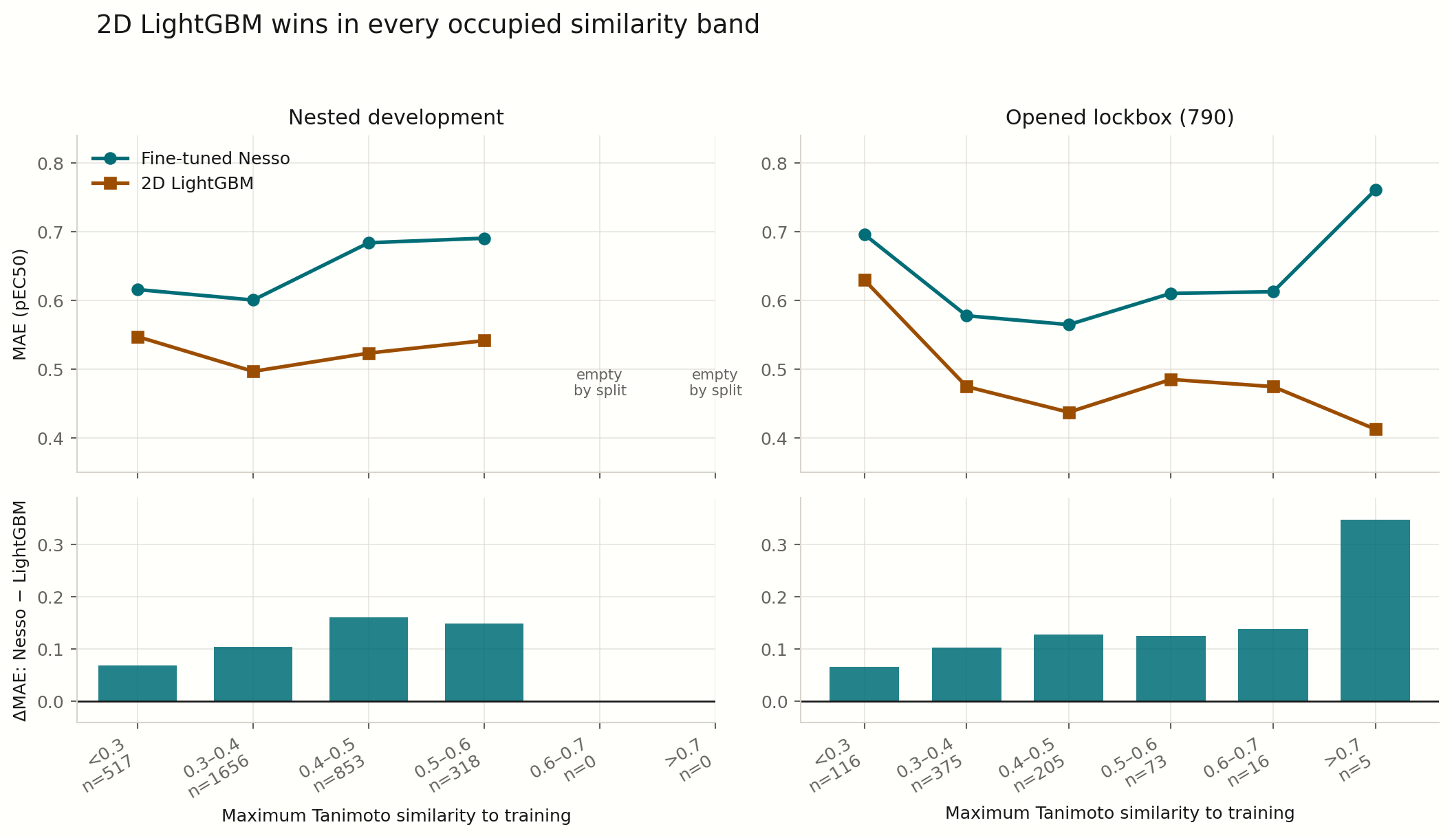
Performance versus chemical distance. Positive ΔMAE means Nesso is worse. LightGBM won in every occupied band. Development has no compounds above 0.60 by construction; the final opened-set bin contains only five compounds.

Model choice stayed inside each outer training set

For every outer fold, learning rate, stopping, and other supervised choices used only the remaining four chemical-family folds. The outer validation labels were not used for tuning. Seeds 42, 43, and 44 were fit after selection and averaged.

The 2D comparator followed the same boundary for supervised steps. Its 14,325-column variance/correlation prefilter was fitted once on the original development structures without labels and then held fixed. Feature ranking to the top 1,000 columns and boosting duration were selected again inside each outer training partition.

The 790 compounds began as a separate historical check set. Once opened, they stopped being a lockbox. I label every analysis on those rows as retrospective and do not use it to justify a new model-selection claim.

Main comparison

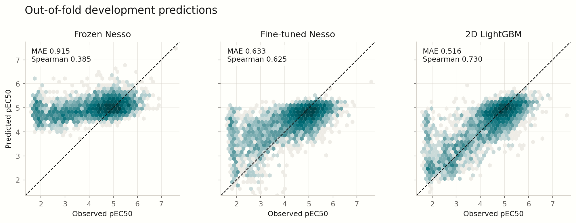
Nested development predictions on shared axes. Fine-tuning repairs the released Nesso score, but LightGBM remains tighter. Both learned models compress the active tail.

Model	Dev MAE	Dev Spearman	Opened 790 MAE	Opened 790 Spearman
Frozen Nesso score	0.915	0.385	0.815	0.312
Affine calibration only	0.839	0.383	0.811	0.312
Fine-tuned Nesso heads	0.633	0.625	0.597	0.581
2D LightGBM	0.516	0.730	0.489	0.697

The development numbers are nested out-of-fold estimates. The LightGBM value on the opened set comes from a later development-selected refit, so it is a retrospective comparison rather than a simultaneous blind test.

Where did the transferable information live?

I froze Nesso’s mean 384D representation and fitted three nested probes: ridge regression, a one-hidden-layer MLP, and a two-hidden-layer MLP.

Readout	Dev MAE	Dev Spearman	Opened 790 MAE	Opened 790 Spearman
Ridge on mean 384D	0.633	0.654	0.596	0.619
One-hidden-layer MLP	0.624	0.645	0.569	0.613
Two-hidden-layer MLP	0.620	0.636	0.576	0.602
Released twin heads, fine-tuned	0.633	0.625	0.597	0.581

The small nonlinear MAE gains over ridge were unresolved at 95% confidence, while their ranking was worse. The clean conclusion is that the frozen representation contains transferable PXR signal and a linear readout recovers most of what these probe classes found. The released output mapping is where transfer failed first.

Did Nesso use the protein?

PXR is constant across all rows, so ordinary fine-tuning cannot answer that question. I tested one narrower mechanism: do the post-pairformer receptor–ligand cells add useful information to the final pooled representation?

I reran Nesso and created three matched 384D vectors after the affinity pairformer:

1. all receptor–ligand and ligand–ligand cells, matching the released average;
2. ligand–ligand cells only;
3. receptor–ligand cells only.

The same frozen output projection and nested ridge protocol were used for all three. All 4,134 compounds completed, the all-pairs vectors reproduced the historical cache, and released-head scores matched to numerical precision.

Final pair pool	Dev MAE	Dev Spearman	Opened 790 MAE	Opened 790 Spearman
All pairs	0.633	0.654	0.596	0.619
Ligand–ligand only	0.606	0.672	0.594	0.631
Receptor–ligand only	0.631	0.642	0.596	0.623

Removing the direct receptor–ligand cells improved development MAE by 0.0266 pEC50 (paired chemical-family bootstrap interval −0.0419 to −0.0114). The opened-set change was unresolved.

This is a late pooling ablation, not a protein-free model and not a protein-causality test. The retained ligand–ligand cells have already passed through protein-conditioned upstream layers. Stronger controls would mask cross-block information before the pairformer, shuffle PXR embeddings, use a matched decoy receptor, and ultimately swap proteins in a multi-target dataset.

The learning-rate boundary was a real protocol flaw

The original grid stopped at 3e-4, and every outer fold selected that boundary. I reran the inner search through 1e-1 at three weight decays.

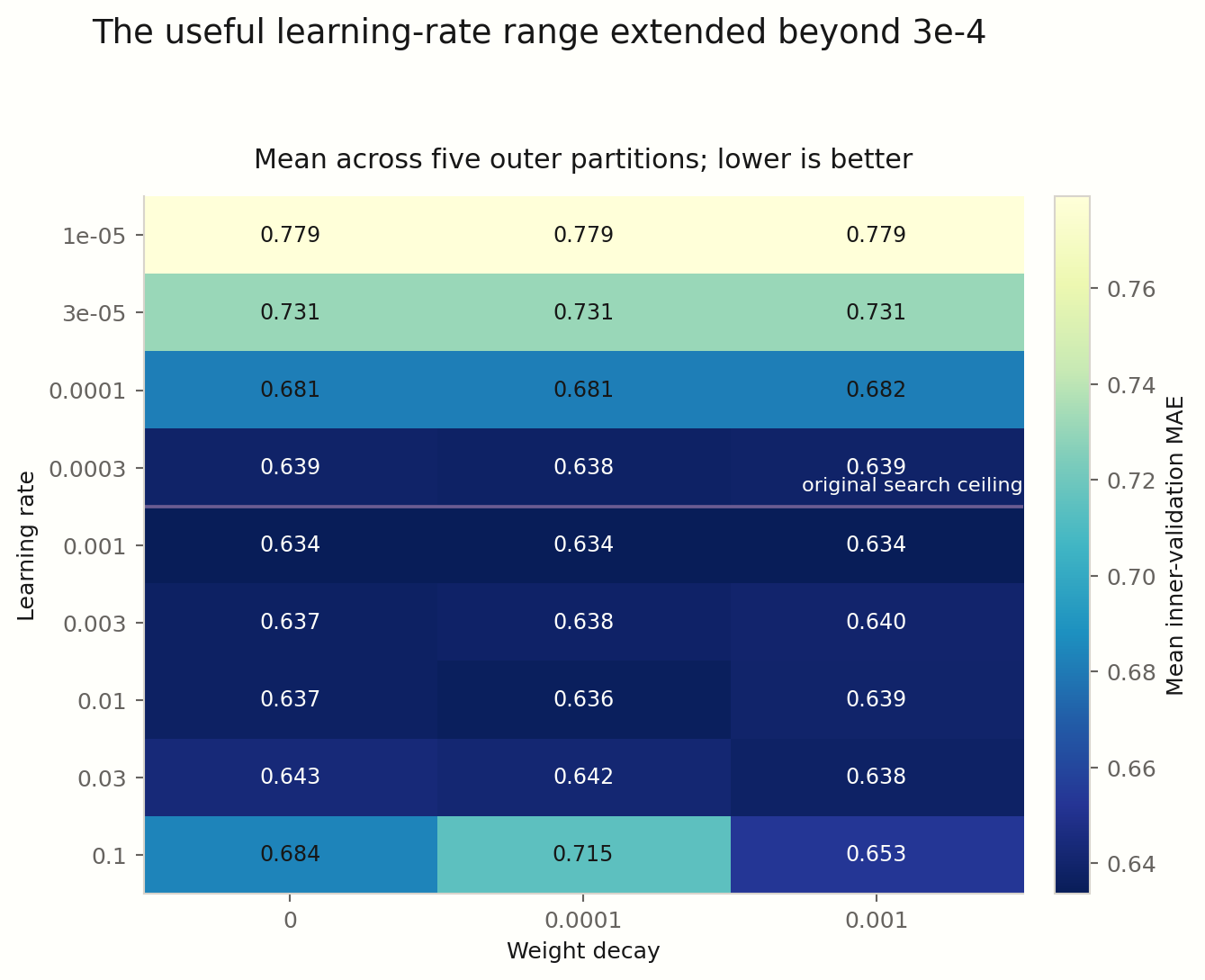
Learning rate × weight decay. The useful region begins around 1e-3 and degrades at 1e-1. Fold-specific selections were 3e-3, 1e-2, 3e-3, 1e-3, and 1e-3.

The expanded search produced nested MAE 0.6345 versus 0.6330 historically. The difference was +0.0016 pEC50, with a paired family-bootstrap interval of −0.0046 to +0.0074. The criticism was right: the initial search was under-bounded. The hypothesis that a larger rate would improve held-out performance was not supported.

This is a protocol-repair sensitivity analysis on previously used development folds, not new confirmation.

What did the twin-head objective do?

The released objective put 50% of the loss on the mean prediction and 25% on each individual head. That is auxiliary per-head supervision, not an explicit consistency penalty. I reran the historical recipes using only the mean-prediction term.

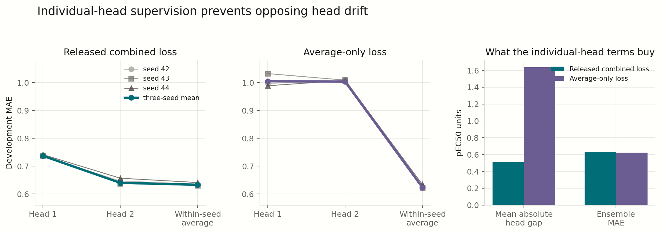
Without individual-head terms, the two heads drift in opposite directions. Their average remains useful, but either head alone becomes poor. The released loss stabilizes the components; it did not improve the averaged prediction used at inference.

The released objective reduced mean head disagreement from 1.637 to 0.508 pEC50. However, average-only training improved ensemble MAE from 0.633 to 0.623. The auxiliary terms solved a real symmetry problem but slightly hurt the quantity that mattered.

Training on 6 − pEC50 only preserved the released score’s numerical orientation. For a symmetric Huber loss it is exactly equivalent to direct pEC50 training after negating and shifting the final linear layer; losses and gradients matched numerically.

Huber δ = 0.5 was a heuristic, not an assay-derived constant. It corresponds to a 3.16-fold concentration error, 3.27 times the median reported assay standard error, and about one third of the development pEC50 interquartile range. Sweeps over MSE, MAE, and Huber deltas did not repair the active tail.

Was pretraining more data-efficient?

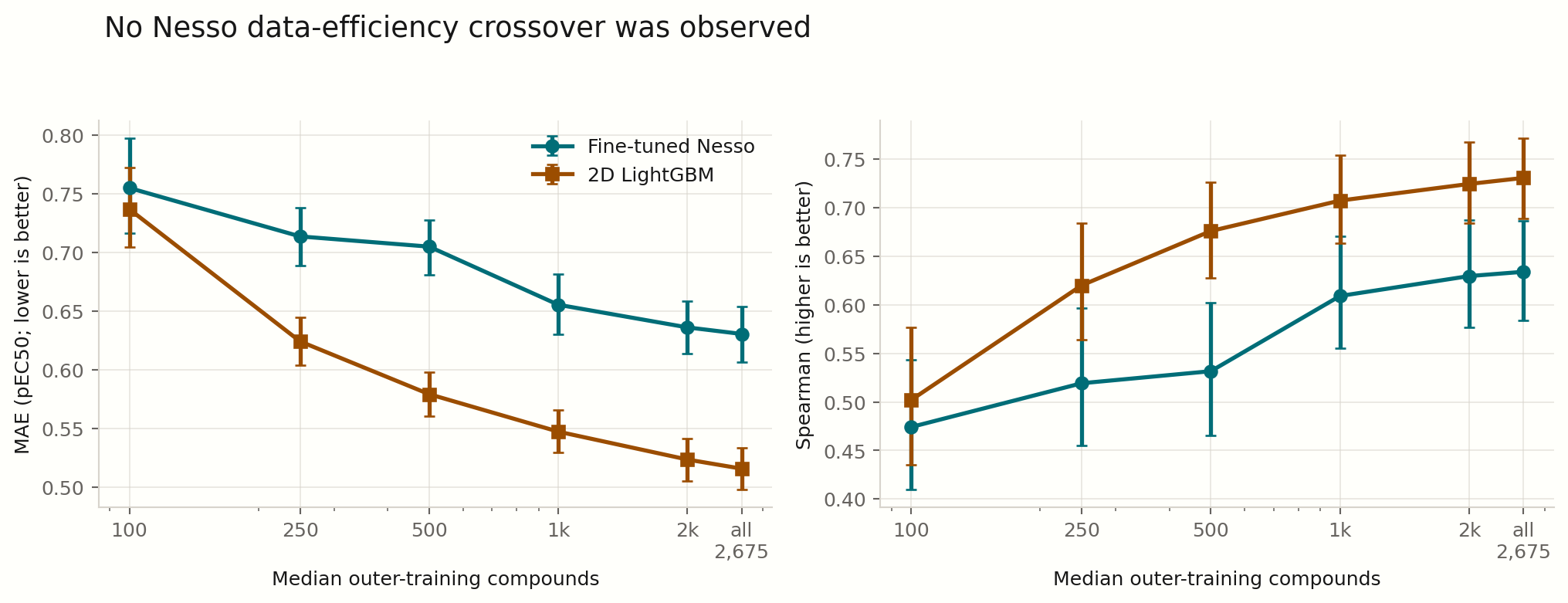
Both models saw the same label-blind chemical-family subsets. At 100 compounds the MAE difference was unresolved, but Nesso’s point estimate was not better. From 250 compounds onward, LightGBM’s advantage was clear.

There was no small-data crossover at the tested sizes. Each size used one deterministic family subset per outer fold, not repeated subset draws. The intervals quantify evaluation-family uncertainty; they do not capture sensitivity to which training families happened to be sampled or to a different clustering threshold.

The shared failure: active-tail compression

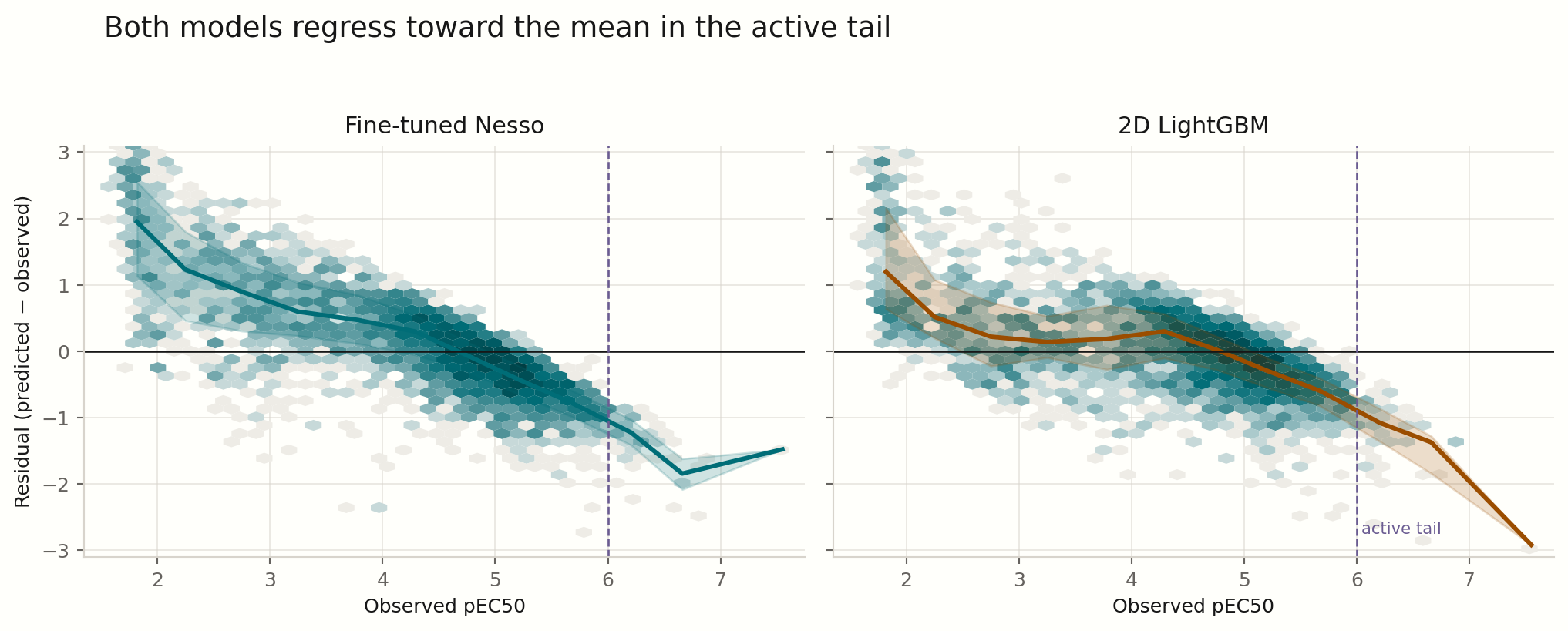
Residual is prediction minus observation. The upward bias at low activity and downward bias at high activity expose regression toward the mean.

Only 55 development compounds had pEC50 above 6. Fine-tuned Nesso predicted one of them above 6; LightGBM predicted none. Loss and learning-rate sweeps did not remove this compression.

The pattern is consistent with label scarcity and regression toward the mean, but the current dossier does not stratify labels by assay batch, curve quality or censoring, partial efficacy, or cytotoxicity and interference flags. I cannot assign the compression uniquely to model bias or Huber loss.

What I take from this

Nesso-1 transferred. The strongest evidence is not the nonlinear fine-tune; it is the ridge probe on a frozen representation. That makes the result easier to defend and cheaper to reproduce.

The structure-aware story is still open. Direct receptor–ligand cells at the tested final pooling point did not help, but that intervention cannot remove protein information already mixed upstream. A stronger protein counterfactual is the highest-value next experiment.

The 2D model remains the practical baseline. A retrospective residual model found a small ranking gain from Nesso features, but its MAE gain was unresolved and the check set was already open. That rule should be frozen and tested once on genuinely new chemistry before it becomes a result.